Train Localization in CBTC: Tachometer + Doppler + Beacon Fusion

When a 600-tonne metro train enters a Communications-Based Train Control (CBTC) zone at 80 km/h, the wayside Zone Controller does not measure where the train is. The train measures where the train is, and reports that measurement up the radio link every cycle. This is the inversion that makes CBTC work — and it works only because the onboard localization stack maintains ±2 to ±5 meter position accuracy continuously, kilometer after kilometer, between balise reads. The stack is a sensor fusion problem in three layers: wheel tachometers and accelerometers integrate continuously, Doppler radar provides slip-immune speed truth, and trackside balises supply absolute position resets every 50 to 200 meters. The Kalman filter that fuses them is the algorithm every CBTC engineer should be able to sketch on the back of a napkin. This article walks through the math, the failure modes, and the engineering choices that determine whether a US transit retrofit lives at the ±2 m or the ±10 m accuracy floor.

Why localization is the accuracy that becomes capacity

Manuscript Chapter 4.2 frames the relationship between localization and headway directly: a CBTC system with ±2-meter positioning accuracy can authorize tighter following distances than one with ±10-meter accuracy because the braking distance calculation is more precise. Position accuracy is not a peripheral subsystem; it is the foundation on which CBTC economics rest. Systems aiming for 90-second or shorter headways generally require ±2 to ±3 meter accuracy at 95 percent confidence; longer-headway systems may tolerate ±5 meters. The cost-benefit trade is explicit — higher accuracy buys tighter headways and higher capacity but requires more sensors, more sophisticated algorithms, and more trackside infrastructure. This article is for the signaling engineer, ATP architect, system integrator, and Independent Safety Assessor who need to understand each sensor’s contribution and how the stack handles failures. Depth lives in Chapter 4 of Communications-Based Train Control, Volume 1.

Layer 1: tachometers and the wheel-diameter problem

The wheel tachometer is the foundation. An inductive or magnetic sensor on a non-driven axle detects each wheel rotation and produces a pulse train. Counting pulses over time yields instantaneous wheel speed; integrating speed yields distance traveled. Most metro fleets carry two to four tachometers per train, one per bogie.

Tachometer odometry has two error sources. The first is wheel-diameter calibration. Distance per wheel rotation depends on wheel circumference; as wheels wear in service, diameter decreases gradually. A 0.1 mm reduction per 1000 km accumulates measurable error. Manuscript Chapter 4.2 quantifies it: over 100 km of travel, a 1 mm wheel-diameter error produces about 300 meters of position drift. The fix is firmware calibration that tracks measured-versus-actual distance and adjusts the tachometer scaling continuously. A well-tuned system holds tachometer scaling error to about ±0.5 percent — 50 meters of error per 10 km traveled.

The second error source is wheel slip and slide. Under heavy braking or acceleration, driven wheels slip relative to the rail, breaking the relationship between rotation and distance. Slip during a 10-second emergency brake application can produce errors exceeding 10 meters. Tachometer-only localization cannot detect slip; the cross-check has to come from another sensor, which is the role of Doppler radar.

Layer 2: Doppler radar as the slip-immune truth source

A Doppler radar mounted under the train measures ground speed by emitting a low-power microwave signal toward the trackbed and reading the frequency shift of returned reflections. The shift is proportional to the radial component of the train’s ground velocity. The output is an instantaneous, slip-independent ground speed measurement at typically 100 Hz update rate.

Manuscript Chapter 4.2 puts Doppler radar accuracy at ±0.1 to 0.5 percent of measured speed, with no mechanical wear (no moving parts) and all-weather operation (rain, snow, mud, darkness). The bias errors are small enough that integrated to position over 10 km, Doppler-only odometry produces 10 to 50 meters of drift — already substantially better than tachometer-only.

The price is hardware cost. A 2D Doppler radar suitable for CBTC applications runs $8,000 to $15,000 per train at 2024 pricing, against $200 to $500 per wheel tachometer. New US CBTC orders typically specify Doppler radar; retrofit projects on legacy fleets often retain wheel-tachometer-only odometry because of the cost and complexity of bogie modification. The MTA’s Second Avenue Subway extension (Phase 2, in design) and the proposed BART Silicon Valley extension specify Doppler radar; the L Line and 7 Line retrofits relied on tachometer-led odometry with later upgrades.

The advantage Doppler brings to fusion is not just better accuracy. It is independence from the failure modes of tachometers. Wheel slip degrades tachometer output; Doppler is unaffected. Wheel wear degrades tachometer scaling; Doppler is unaffected. The two sensors fail in different ways, which is what fusion exploits.

Layer 3: accelerometers and inertial measurement

A three-axis accelerometer (or a full Inertial Measurement Unit combining accelerometers and gyroscopes) measures longitudinal, lateral, and vertical acceleration directly. Double-integrated, acceleration produces speed and distance. Over short intervals, inertial measurement is very accurate; over longer intervals, drift accumulates rapidly and integration becomes unusable.

The role of the accelerometer in a CBTC localization stack is not primary localization. It is slip detection (the vertical acceleration signature of a wheel slip event is distinctive), grade compensation (a 2 percent grade introduces a 0.2 m/s² longitudinal acceleration component that has to be distinguished from actual motion), and sensor-fusion confidence (the accelerometer’s independent acceleration estimate cross-checks tachometer and Doppler agreement during transients).

A quality MEMS IMU costs $1,000 to $3,000 and is typically co-located with the Doppler radar as an integrated sensor package.

Layer 4: balises as the absolute position reset

Odometry alone cannot sustain ±2 to ±5 meter accuracy over kilometers. After 10 km of travel, even a well-tuned tachometer-Doppler-IMU stack accumulates ±50 to ±100 meters of uncertainty. After 50 km, uncertainty can exceed ±300 to ±500 meters. The localization stack needs periodic absolute position references, and trackside balises provide them.

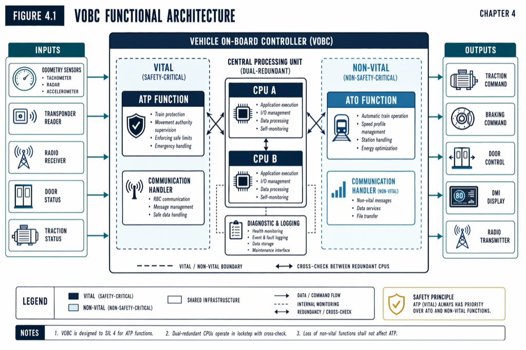
A balise is a small, passive transponder buried beneath the track surface. When a balise antenna under the train passes over the balise, the antenna’s induced electromagnetic field powers the balise, which transmits a unique identifier and a brief data payload. The Vehicle On-Board Controller (VOBC) records the transponder ID, looks up the corresponding known position from the onboard track database, and resets the localization estimate. Accumulated odometric drift collapses to the balise’s intrinsic position uncertainty — typically ±0.5 meters.

Manuscript Chapter 4.2 covers the balise types and spacing decisions. Passive balises (Eurobalise pattern) are most common in modern deployments — no battery, no power supply, 30+ year service life, $900 to $1,700 per unit installed. Active balises ($3,000 to $8,000 per unit) offer longer read range and bidirectional communication but require power and periodic battery replacement; they are used in extreme environments. Spacing typically runs 50 to 200 meters depending on the headway target. Denser placement (50 m) caps drift accumulation tightly and supports aggressive headway targets; sparser placement (150 to 200 m) reduces infrastructure cost on lower-capacity lines.

The Kalman filter: how the four layers become one estimate

No single sensor is sufficient. The fusion algorithm is a Kalman filter — a recursive Bayesian estimator that optimally combines noisy measurements to produce the best estimate of true position and speed.

The filter operates in three steps every cycle. Predict. Using the previous position and speed estimate plus the process model (constant velocity with acceleration noise, modified by gradient and curvature from the track database), predict the current position and the associated covariance.

Update. Incorporate the latest measurements — tachometer pulse count, Doppler speed, accelerometer integration, balise read if one occurred — by computing the Kalman gain (which measurement to trust more), updating the position estimate toward the measurements weighted by their inverse covariances, and shrinking the covariance accordingly.

Project. The updated position and speed estimate, with its current uncertainty bound, is reported to the VOBC safety logic and to the wayside Zone Controller as the position payload of the next heartbeat report.

The Kalman gain is the heart of the filter. A well-tuned filter automatically downweights sensors that are producing outliers (a malfunctioning tachometer reporting wildly inconsistent counts, for example) and emphasizes sensors that agree. After a balise read, the position covariance shrinks sharply to about ±0.5 m; between reads, it grows according to the dominant odometric drift mode. Manuscript Chapter 4.2 puts well-tuned filter performance at ±1 to ±2 meter accuracy maintained over 10 to 20 km between balise updates.

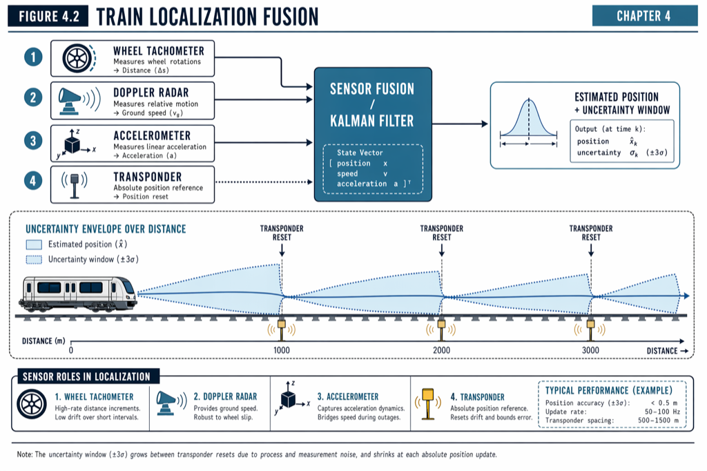The sawtooth: position uncertainty grows between balise reads, collapses to about ±0.5 m at each read. Balise spacing sets the upper bound on uncertainty between reads.

Failure modes and graceful degradation

The four-layer stack is engineered to fail gracefully. Three failure modes matter most.

Single tachometer fault. A tachometer reporting outliers (wheel slip or sensor degradation) is downweighted by the Kalman filter automatically. The remaining tachometers, Doppler, accelerometer, and balise reads continue to provide position with marginal accuracy degradation. The fault is logged for maintenance.

Doppler radar fault. Loss of Doppler removes the slip-immune cross-check. The system falls back to tachometer-led fusion, which still works but is more vulnerable to wheel slip during heavy braking. Typical CBTC implementations continue normal operation but flag the fault for maintenance and may impose a small additional safety margin in the EBD calculation.

Balise read miss. If a train passes over a balise but does not register a read (antenna fault, balise damage, RF interference), the filter does not reset and uncertainty continues to accumulate. After several missed reads in sequence, uncertainty grows beyond the safe operating threshold (typically ±20 to ±50 meters) and the system requires re-initialization. Manuscript Chapter 4.2 documents re-initialization procedures: limp-home mode at reduced speed (10 to 20 km/h) under driver command, with the train relying on subsequent balise reads to constrain uncertainty.

The catastrophic failure mode is loss of all odometric sensors simultaneously — tachometer, Doppler, and accelerometer all silent. This produces a localization-unknown state, and the only recovery is either a balise read (which provides absolute position) or manual positioning entry by a supervisor. Most CBTC implementations require the train to be stopped before re-initialization in this state.

Map matching and the track database

Train position is meaningful only against track geometry. The onboard track database stores the entire line geometry: track centerlines, switch positions, station stop locations, speed restrictions, balise locations, and grade and curvature profiles. Manuscript Chapter 4.2 puts a typical metro line database at 10 to 50 MB.

Map matching is the algorithm that projects the Kalman-filtered position estimate onto the track centerline. The constraint that trains operate on fixed tracks reduces the localization problem from two-dimensional (or three) to one-dimensional (along-track distance from a reference point). If the filter reports an estimate 0.5 meters off the track centerline, map matching corrects the estimate onto the centerline and updates the lateral uncertainty. In tunnels and underground sections where GNSS is unavailable, map matching is often the dominant source of large-scale verification.

Database management is a configuration management problem (covered in Change Orders on CBTC Projects: Why They Happen, How to Bound Them). The VOBC operates dual-database capability: the active database while a new version is loaded into secondary memory, validated for geometric consistency, and only then marked active. A corrupted or misconfigured database is one of the most common late-project surprises in US CBTC retrofits.

Why the math compounds into capacity

Manuscript Chapter 4.3 documents that improving position accuracy from ±20 m to ±10 m yields 8 to 12 seconds of headway margin or permits higher speeds on curves on a 90-second-headway line. The mechanism is straightforward: position uncertainty drives the Supervised Location offset, which extends the EBD, which forces wider headways. Tightening the localization accuracy band by 10 meters tightens the EBD by 10 meters, which on a 90-second-headway design recovers proportional capacity.

This is why localization sensor specification is one of the most-leveraged decisions in a CBTC RFP. A retrofit that specifies tachometer-only odometry on a legacy fleet locks the system to the ±15 to ±20 meter accuracy band; the same retrofit specifying Doppler radar plus IMU plus 100-meter balise spacing reaches the ±5 to ±10 meter band. The headway difference between the two specifications is measurable in the line’s capacity for the next 25 years.

The four-layer localization stack: continuous odometry, slip-immune cross-check, slip detection, absolute reset. The Kalman filter is the integration point.

Practical takeaways

• Tachometers, Doppler radar, accelerometer, and balises are not redundant; they are complementary. Each fails in a different way; the fusion algorithm exploits the diversity to produce ±1 to ±2 m accuracy that no single sensor can deliver alone.
• Wheel-diameter calibration error is the dominant tachometer error mode. A 1 mm error produces 300 m of drift over 100 km. Firmware calibration is a continuous, ongoing maintenance task.
• Doppler radar buys slip immunity and ±0.1 to 0.5 percent speed accuracy, at $8,000 to $15,000 per train installed. The cost-benefit is straightforward for new builds; retrofit decisions depend on bogie modification feasibility.
• Balise spacing (50 to 200 meters) is a deliberate trade between infrastructure cost and headway capacity. Denser spacing caps drift accumulation tightly; sparser spacing relies more on odometric quality.
• The Kalman filter is the integration point. A well-tuned filter holds ±1 to ±2 m accuracy between balise updates over 10 to 20 km. Tuning is a commissioning activity that has to be revisited as wheels wear and Doppler bias drifts.

Where to go next

This post is an 11-minute walkthrough of the localization stack. The full treatment, including the worked Kalman filter mathematics, the dark-start initialization procedures, the balise placement strategy, and emerging GNSS and visual odometry technologies, lives in Chapter 4 (Onboard Equipment), section 4.2, of Communications-Based Train Control, Volume 1: Foundations & Technical Architecture (Buy on Amazon). Download Chapter 4 slides (free PDF) for the localization architecture diagrams.

For the broader picture of what the VOBC does with the position estimate, see The Onboard Side of CBTC: Inside the VOBC. For how localization accuracy translates into braking distance and headway, see Inside the CBTC Braking Curve: How Safe Stopping Distance Is Calculated.

Sources

• Wang, C. (2026). Communications-Based Train Control, Volume 1: Foundations & Technical Architecture. Independent. ISBN 979-8-258-54295-3. — Chapter 4, “Onboard Equipment,” section 4.2.
• IEEE Standards Association. IEEE Std 1474.1: Communications-Based Train Control (CBTC) Performance and Functional Requirements.
• IEEE Standards Association. IEEE Std 1474.4: Recommended Practice for Functional Tests of a Communications-Based Train Control (CBTC) System.
• European Union Agency for Railways. Subset-036: FFFIS for Eurobalise. era.europa.eu
• International Electrotechnical Commission. IEC 62290-1: Railway applications — Urban guided transport management and command/control systems.
• Federal Transit Administration. (2016). FTA Report No. 0045: Communications-Based Train Control (CBTC) Technology. transit.dot.gov
• MTA New York City Transit. Communications-Based Train Control Status Update. new.mta.info/project/communications-based-train-control-cbtc